With strong earning rates on everyday spending, flexible Chase Ultimate Rewards points and a modest $95 annual fee, it delivers outsize value for beginners (as well as seasoned travelers). Plus, Chase just introduced several new earning rates and perks to the card, providing more value to cardholders without raising the annual fee.
Below, we’ll break down its current bonus, ongoing perks and why the Sapphire Preferred continues to earn a spot in so many travelers’ wallets.
Chase Sapphire Preferred current offer
New Sapphire Preferred cardholders can earn 100,000 bonus points after spending $5,000 on purchases in the first three months from account opening.
According to our June 2026 valuations, this offer is worth up to $2,050.
Now is an excellent time to get the Sapphire Preferred, since the welcome offer alone provides more than $2,000 in value thanks to its valuable transferable rewards.
Chase Ultimate Rewards points are among the most valuable transferable currencies available, thanks to a robust roster of airline and hotel partners and high-value redemption options.
The Chase Sapphire Preferred has many generous bonus-earning categories. Plus, the card has recently announced two new bonus categories, along with an enhancement to its Chase Travel℠ category.
You’ll earn:
5 points per dollar spent on all Chase Travel purchases, including flights, hotels, rental cars, vacation homes*, cruises, activities and tours
5 points per dollar spent on Lyft (through Sept. 30, 2027)
5 points per dollar spent on eligible Peloton equipment and accessory purchases over $150 (through Dec. 31, 2027)
*New category ^Vacation home brands included in this category: Airbnb, Vrbo, Plum Guide, HomeAway, Homestay.com and Vacasa
CHRIS DONG/THE POINTS GUY
The Sapphire Preferred has also increased its annual hotel statement credit, doubling it from $50 to $100. The credit can be used for prepaid hotel stays booked through Chase Travel and is available each account anniversary year.
New cardholders who apply on or after June 15 will no longer be eligible for the Sapphire Preferred’s 10% annual points bonus.
However, new and current cardholders will receive two new perks:
A one-year complimentary Apple TV subscription (when activated by Dec. 31)
Up to $120 in statement credits for Global Entry, TSA PreCheck or Nexus every four years
Cardholders will also receive a complimentary DoorDash DashPass membership (a value of $120 per year) and a monthly $10 credit for eligible non-restaurant DoorDash purchases.
It’s important to note that Chase is reducing the World of Hyatt transfer ratio. If you apply on or after June 15, transfers to World of Hyatt will occur at a 4:3 ratio instead of 1:1, resulting in fewer Hyatt points for the same number of Ultimate Rewards points transferred. Existing cardholders and those who applied before June 15 can continue transferring at the 1:1 ratio until Oct. 1.
Despite the Hyatt transfer change, Ultimate Rewards points remain highly valuable thanks to Chase’s airline and hotel partners, which can unlock aspirational business-class tickets or picturesque stays at island resorts for far less than their cash equivalent.
The Sapphire Preferred remains one of the top travel rewards credit cards on the market. Its current 100,000-point welcome bonus matches the highest offer we’ve seen in the card’s history, making now an excellent time to add it to your wallet.
Despite the Hyatt transfer devaluation, the Sapphire Preferred’s latest changes to earning rates and statement credits are a net positive overall — especially considering its annual fee remains unchanged at $95.
It’s no wonder so many TPG staffers continue to carry the Sapphire Preferred year after year. Given its easy-to-maximize perks, strong earning rates and valuable Ultimate Rewards points, it deserves a place in any traveler’s wallet.
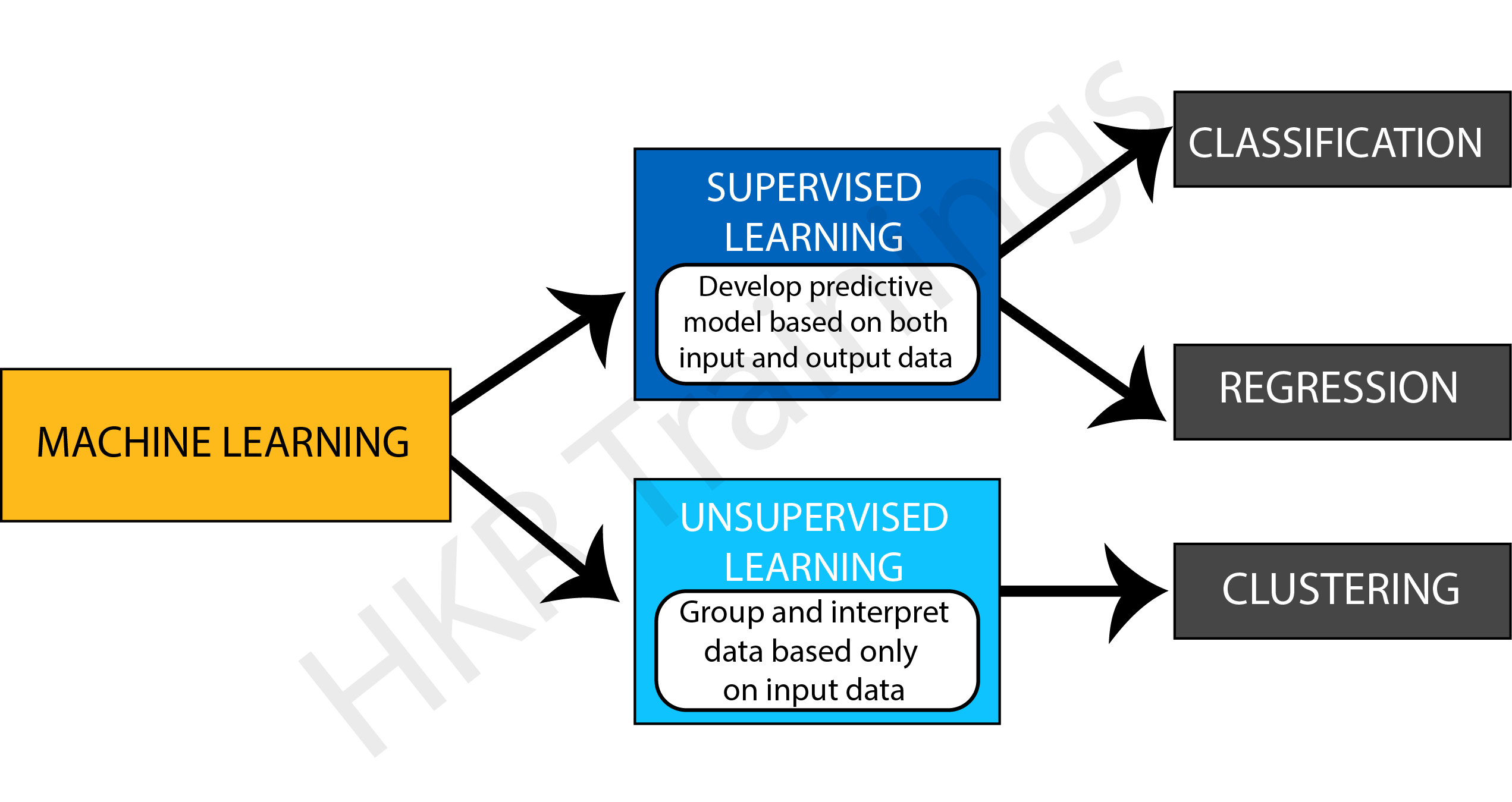
The Classification algorithm is a supervised learning method that trains data to determine the category of future observations. This is why firstly, let us understand what is supervised learning.
What is Supervised Learning
Supervised learning develops a function to predict a defined label based on the input data.
The model in Supervised Learning learns by action. During training, the model examines which label is related to the given data and, as a result, can identify patterns between the data and particular labels.
Let us understand supervised learning with an example of Speech Recognition. It is an application where you train an algorithm with your voice. Virtual assistants such as Google Assistant and Siri, which recognize and respond to your voice, are the most well-known real-world supervised learning applications.
Supervised Learning might sort data into categories (a classification challenge) or predict a result (regression algorithms). This article will specifically address everything we need to know about classification in Machine Learning.
What is Classification in Machine Learning?
The process of recognizing, interpreting, and classifying objects or thoughts into various groups is known as classification. Machine learning models use a variety of algorithms to classify future datasets into appropriate and relevant categories with the help of already-categorized training datasets.
In other words, classification is a type of “pattern recognition.” In this case, classification algorithms applied to training data detect the same pattern (same number sequences, words, etc.) in consecutive data sets.
There are four primary classification tasks you could come across:
Binary Classification
Multi-Class Classification
Multi-Label Classification
Imbalanced Classification
Binary Classification
The term “binary classification” refers to tasks that can provide one of two class labels as an output. In general, one is regarded as the normal state, while the other is abnormal. The following examples can assist you in better comprehending them.
For example, for email spam detection, the normal condition is “not spam,” whereas the abnormal state is “spam.” “Likewise, Cancer not found” is the normal condition of an activity involving a medical test, whereas “cancer identified” is the abnormal state.
The normal state class is usually allocated the class label 0, whereas the abnormal state class is assigned the class label 1.
Some of the popular algorithms used for binary classification are:
Decision Trees
Logistic Regression
Support Vector Machine
k-Nearest Neighbors
Naive Bayes
Machine Learning Training
Master Your Craft
Lifetime LMS & Faculty Access
24/7 online expert support
Real-world & Project Based Learning
Multi-Label Classification
We refer to multi-label classification tasks as those in which we need to assign two or more distinct class labels that can be predicted for each case. A simple example is photo classification, in which a single shot may contain many items, such as a puppy or an apple, and so on. In this type of classification, you can predict many labels rather than just one.
The most common algorithms are:
Multi-label Random Forests
Multi-label Decision trees
Multi-label Gradient Boosting
Multi-Class Classification
Tasks that have two or more class labels are called multi-class classification.
The multi-class classification does not differentiate between normal and abnormal results.
In some situations, the number of class labels might be rather big. For instance, a model may predict that a photograph belongs to one of thousands or tens of thousands of faces in a facial recognition system. Examples are classified into one of several known classes.
Some of the popular algorithms used for multi-class classification are:
Naive Bayes
k-Nearest Neighbors
Random Forest
Gradient Boosting
Decision Trees
Imbalanced Classification
Imbalanced Classification refers to tasks in which the number of items in each class is distributed unequally. In general, unbalanced classification problems are binary classification tasks in which most of the training dataset belongs to the normal class and just a small percentage to the abnormal class.
Learners in Classification Problem
There are two types of learners in a classification problem, namely:
Eager Learners
Lazy Learners
Eager Learners
Eager learning occurs when a machine learning algorithm constructs a model shortly after obtaining training data. It’s named eager because the first thing it does when it obtains the data set is, it creates the model. The training data is then forgotten. When new input data arrives, the model is used to evaluate it. The vast majority of machine learning algorithms are eager to learn.
Lazy Learners
Lazy learning, on the other hand, occurs when a machine learning algorithm does not develop a model immediately after receiving training data but instead waits until it is given input data to analyze. It’s named lazy because it waits until it’s absolutely essential to construct a model if it builds any at all. It only saves training data when it receives it. When the input data arrives, it uses the previously stored data to evaluate the output. Instead of learning a discriminative function from the training data, the lazy learning algorithm “memorizes” the training dataset. The eager learning algorithm, on the other hand, learns its model weights (parameters) during training.
Types of Machine learning Classification Algorithms
Classification algorithms use input training data in machine learning to predict the likelihood or probability that the following data will fall into one specified category. One of the most popular classifications used to sort emails into “spam” and “non-spam” categories, as employed by today’s leading email service providers.
They are two types of classification models, namely:
Linear Models
Non-linear Models
1. Linear Models
Support Vector Machine
The support vector machine (SVM) is a frequently used machine learning technique for classification and regression problems. It is, however, mostly employed to tackle categorization difficulties. SVM’s main goal is to determine the best decision boundaries in an N-dimensional space that can classify data points, and the optimal decision boundary is known as the Hyperplane. The extreme vector is chosen by SVM to locate the hyperplane, and these vectors are referred to as support vectors.
Logistic Regression
In logistic regression, the sigmoid function returns the probability of a label. It is used widely when the classification problem is binary, for example, true or false, win or lose, positive or negative.
Logistic regression is used to determine the right fit between a dependent variable and a set of independent variables. Because it quantifies the factors that lead to categorization, it beats alternative binary classification algorithms like KNN.
Subscribe to our YouTube channel to get new updates..!
2. Non-Linear Models
Decision Tree
The classification model is developed using the decision tree algorithm as a tree structure. The data is then divided down into smaller structures and connected to an incremental decision tree to complete the process. The final output looks like a tree, complete with nodes and leaves. Using the training data, the rules are learned one by one, one by one. Every time a rule is learned, the tuples that cover the rules are removed. The technique is repeated on the training set until the termination point is reached.
The tree is built using a recursive top-down divide and conquer method. A leaf symbolizes a classification or decision, and a decision node will contain two or more branches. The root node of a decision tree is the highest node that corresponds to the best predictor, and the best thing about a decision tree is that it can handle both category and numerical data.
Kernel SVM
A kernel in SVM is a function that assists in problem resolution. They provide you shortcuts so you don’t have to complete hard calculations. Kernel is remarkable since it allows us to go to higher dimensions and do smooth calculations. It is possible to work with an infinite number of dimensions with kernels.
K-Nearest Neighbor
The K-Nearest Neighbor technique divides data into groups based on the distance between data points and is used for classification and prediction. The K-Nearest Neighbor algorithm implies that data points near together must be similar. Hence, the data point to be classed will be grouped with the closest cluster.
Naive Bayes
The classification algorithm Naive Bayes is based on the assumption that predictors in a dataset are independent. This implies that the features are independent of one another. For example, when given a banana, the classifier will notice that the fruit is yellow in color, rectangular in shape, and long and tapered. These characteristics will add to the likelihood of it becoming a banana in its own right and are not reliant on one another. Naive Bayes is based on the Bayes theorem, which is represented as:
P(A|B) = (P(A) P(B|A)) / P(B)
Here: P(A | B) = how likely B happens P(A) = how likely A happens P(B) = how likely B happens P(B | A) = how likely B happens given that A happen
Stochastic Gradient Descent
It is an extremely effective and simple method for fitting linear models. If the sample data is vast, Stochastic Gradient Descent is beneficial. For classification, it provides a variety of loss functions and penalties.
The only benefit is the ease of implementation and efficiency. Still, stochastic gradient descent has several drawbacks, including the need for many hyper-parameters and sensitivity to feature scaling.
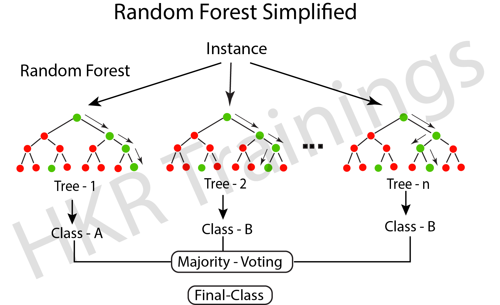
Random Forest
Random decision trees, also known as random forest, may be used for classification, regression, and other tasks. It works by building many decision trees during training and then outputs the class that is the individual trees’ mode, mean, or classification prediction.
A random forest (meta-estimator) fits several trees to different subsamples of data sets and averages the results to increase the model’s predicted accuracy. The sub-sample size is similar to the original input size; however, replacements are frequently used in the samples.
Artificial Neural Networks
A neural network uses a model inspired by neurons and their connections in the brain to convert an input vector to an output vector. The model comprises layers of neurons coupled by weights that change the relative relevance of different inputs. Each neuron has an activation function that controls the cell’s output (as a function of its input vector multiplied by its weight vector). The output is calculated by applying the input vector to the network’s input layer, then computing each neuron’s outputs via the network (in a feed-forward fashion).
Machine Learning Training
Weekday / Weekend Batches
Conclusion
In this blog, we looked at what Supervised Learning is and its sub-branch Classification, some of the most widely used classification models, and how to predict their accuracy and see whether they are trained correctly.
To provide the best experiences, we use technologies like cookies to store and/or access device information. Consenting to these technologies will allow us to process data such as browsing behavior or unique IDs on this site. Not consenting or withdrawing consent, may adversely affect certain features and functions.
Functional
Always active
The technical storage or access is strictly necessary for the legitimate purpose of enabling the use of a specific service explicitly requested by the subscriber or user, or for the sole purpose of carrying out the transmission of a communication over an electronic communications network.
Preferences
The technical storage or access is necessary for the legitimate purpose of storing preferences that are not requested by the subscriber or user.
Statistics
The technical storage or access that is used exclusively for statistical purposes.The technical storage or access that is used exclusively for anonymous statistical purposes. Without a subpoena, voluntary compliance on the part of your Internet Service Provider, or additional records from a third party, information stored or retrieved for this purpose alone cannot usually be used to identify you.
Marketing
The technical storage or access is required to create user profiles to send advertising, or to track the user on a website or across several websites for similar marketing purposes.