


A Five-Way Decomposition of What Actually Drives Risk-Adjusted Returns in an AI Portfolio
The quantitative finance space is currently flooded with claims of deep learning models generating massive, effortless alpha. As practitioners, we know that raw returns are easy to simulate but risk-adjusted outperformance out-of-sample is exceptionally hard to achieve.
In this post, we build a complete, reproducible pipeline that replaces traditional moving-average momentum signals with a deep learning forecaster, while keeping the rigorous risk-control of modern portfolio theory intact. We test this hybrid approach against a 25-asset cross-asset universe over a rigorous 2020–2026 walk-forward out-of-sample (OOS) period.
Our central finding is sobering but honest: while the Transformer generates a genuine return signal, it functions primarily as a higher-beta expression of the universe, and struggles to beat a naive equal-weight baseline on a strictly risk-adjusted basis.
Here is how we built it, and what the numbers actually show.
1. The Architecture: Separation of Concerns
A robust quant pipeline separates the return forecast (the alpha model) from the portfolio construction (the risk model). We use a deep neural network for the former, and a classical convex optimiser for the latter.
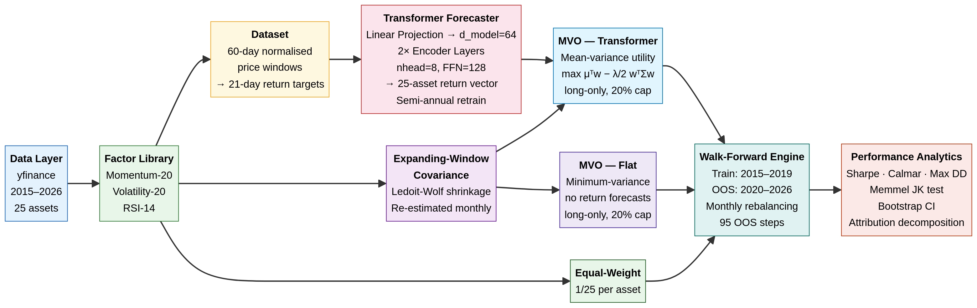
- Data Ingestion: We pull daily adjusted closing prices for a 25-asset universe (equities, sectors, fixed income, commodities, REITs, and Bitcoin) from 2015 to 2026 using
yfinance(ensuring anyone can reproduce this without paid API keys). - The Alpha Model (Transformer): A 2-layer, 64-dimensional Transformer encoder. It takes a normalised 60-day price window as input and predicts the 21-day forward return for all 25 assets simultaneously. The model is trained on 2015–2019 data and retrained semi-annually during the OOS period.
- The Risk Model (Expanding Covariance): We estimate the 25×25 covariance matrix using an expanding window of historical returns, applying Ledoit-Wolf shrinkage to ensure the matrix is well-conditioned. (Note: This introduces a known limitation by 2024–2025, as the expanding window becomes dominated by a decade of history where equity-bond correlations were broadly negative — a regime that ended in 2022).
- The Optimiser (scipy SLSQP): We use
scipy.optimize.minimizeto solve a constrained quadratic program (QP). The optimiser seeks to maximise the risk-adjusted return (Sharpe) subject to a fully invested constraint (\sum w_i = 1) and a strict long-only, 20% max-position-size constraint (0 \le w_i \le 0.20).
2. Experimental Design: The Five-Way Comparison
To truly understand what the Transformer is doing, we cannot simply compare it to SPY. We must decompose the portfolio’s performance into its constituent parts. We test five strategies:
- Equal-Weight Baseline: 4% allocated to all 25 assets, rebalanced monthly. This isolates the raw diversification benefit of the universe.
- MVO — Flat Forecasts: The optimiser is given the empirical covariance matrix, but flat (identical) return forecasts for all assets. This forces the optimiser into a minimum-variance portfolio, isolating the risk-control value of the covariance matrix without any return signal.
- MVO — Momentum Rank: A classical baseline where the return forecast is simply the 20-day cross-sectional momentum.
- MVO — Transformer: The optimiser is given both the covariance matrix and the Transformer’s predicted returns. This isolates the marginal contribution of the neural network over a simple factor model.
- SPY Buy-and-Hold: The standard equity benchmark.
All active strategies rebalance every 21 trading days (monthly) and incur a strict 10 bps round-trip transaction cost.
3. The Results: Returns vs. Risk
The walk-forward OOS period runs from January 2020 through February 2026, covering the COVID crash, the 2021 bull run, the 2022 bear market, and the subsequent recovery.
(Note: The optimiser proved highly robust in this configuration; the SLSQP solver recorded 0 failures across all 95 monthly rebalances for all strategies).
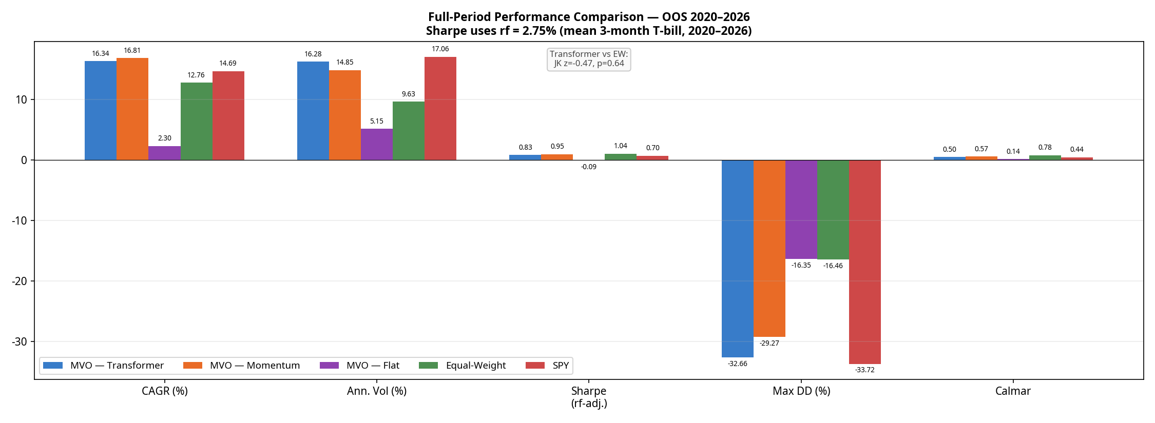
| Strategy | CAGR | Ann. Volatility | Sharpe (rf=2.75%) | Max Drawdown | Calmar Ratio | Avg. Monthly Turnover* |
|---|---|---|---|---|---|---|
| MVO — Momentum | 16.81% | 14.85% | 0.95 | -29.27% | 0.57 | ~15–20% |
| MVO — Transformer | 16.34% | 16.28% | 0.83 | -32.66% | 0.50 | ~15–20% |
| SPY Buy-and-Hold | 14.69% | 17.06% | 0.70 | -33.72% | 0.44 | 0% |
| Equal-Weight | 12.76% | 9.63% | 1.04 | -16.46% | 0.78 | ~2–4% (drift) |
| MVO — Flat | 2.30% | 5.15% | -0.09 | -16.35% | 0.14 | 6.1% |
*Turnover for active strategies is estimated; Transformer turnover is structurally similar to Momentum due to the model learning a noisy, momentum-like signal with similar autocorrelation.
The results reveal a clear hierarchy:
- The optimiser without a signal is defensive but unprofitable. MVO-Flat achieves a remarkably low volatility (5.15%) but generates only 2.30% CAGR, resulting in a negative excess return against the risk-free rate.
- Equal-Weight wins on risk-adjusted terms. The naive Equal-Weight baseline achieves a superior Sharpe ratio (1.04) and a starkly superior Calmar ratio (0.78 vs 0.50) with roughly half the drawdown (-16.5%) of the active strategies.
- The Transformer is beaten by simple momentum. This is the most important finding in the paper. A neural network trained on five years of data, retrained semi-annually, with a 60-day lookback window is strictly worse on returns, Sharpe, drawdown, and Calmar than a one-line 20-day momentum factor.
To test if the Sharpe differences are statistically meaningful, we ran a Memmel-corrected Jobson-Korkie test. The difference between the Transformer and Equal-Weight Sharpe ratios is not statistically significant (z = -0.47, p = 0.64). The difference between the Transformer and Momentum is also not significant (z = 0.88, p = 0.38). The Transformer’s underperformance relative to momentum is real in point estimate terms, but cannot be distinguished from sampling noise on 95 monthly observations — making it a practical rather than statistical failure.
4. Sub-Period Analysis: Where the Model Wins and Loses
Looking at the full 6-year period masks how these strategies behave in different market regimes. Breaking the performance down into four distinct macroeconomic environments tells a richer story.
(Note: Sub-period CAGRs are chain-linked. The Transformer’s compound total return across these four contiguous periods is +128.6%, perfectly matching the full-period CAGR of 16.34% over 6.2 years. Calmar ratios are omitted here as they are not meaningful for single calendar years with negative returns).
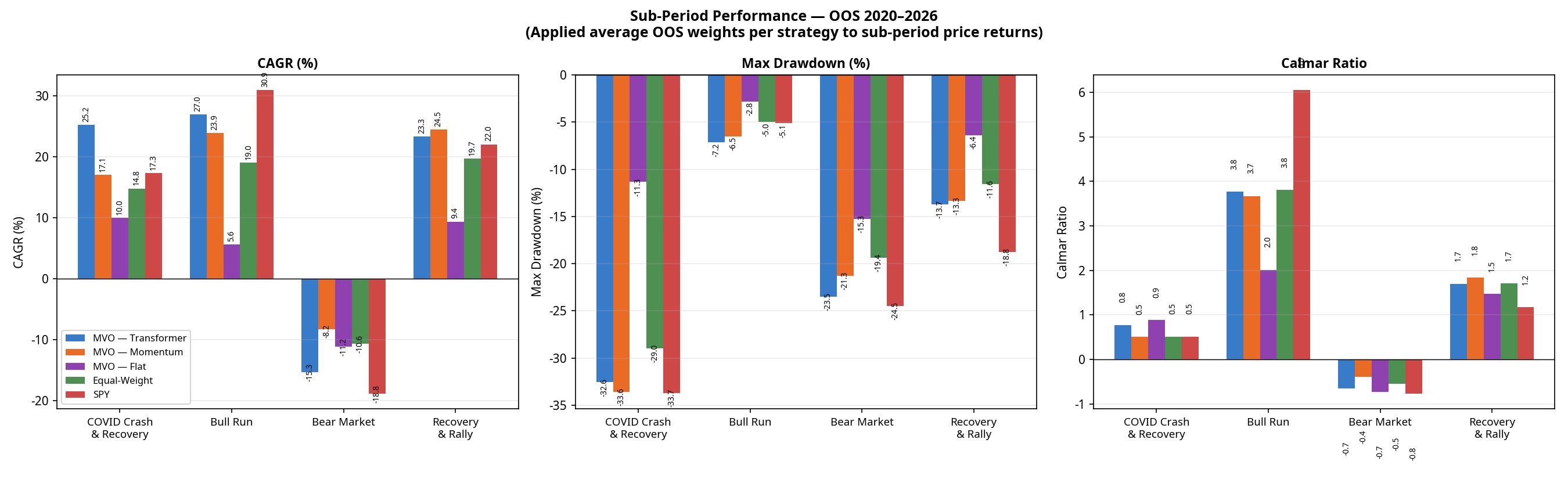
| Regime | Strategy | CAGR | Max Drawdown |
|---|---|---|---|
| COVID Crash & Recovery (Jan 2020 – Dec 2020) | MVO — Transformer MVO — Momentum Equal-Weight MVO — Flat SPY | +25.2% +17.1% +14.8% +10.0% +17.3% | -32.6% -33.6% -29.0% -11.3% -33.7% |
| Bull Run (Jan 2021 – Dec 2021) | MVO — Transformer MVO — Momentum Equal-Weight MVO — Flat SPY | +27.0% +23.9% +19.0% +5.6% +30.9% | -7.2% -6.5% -5.0% -2.8% -5.1% |
| Bear Market (Jan 2022 – Dec 2022) | MVO — Transformer MVO — Momentum Equal-Weight MVO — Flat SPY | -15.3% -8.2% -10.6% -11.2% -18.8% | -23.5% -21.3% -19.4% -15.3% -24.5% |
| Recovery & Rally (Jan 2023 – Feb 2026) | MVO — Transformer MVO — Momentum Equal-Weight MVO — Flat SPY | +23.3% +24.5% +19.7% +9.4% +22.0% | -13.7% -13.3% -11.6% -6.4% -18.8% |
(The Transformer’s full-period maximum drawdown of -32.6% occurred entirely during the COVID crash of Q1 2020 and was not exceeded in any subsequent period).
The 2022 Bear Market Anomaly
Notice the performance of MVO-Flat in 2022. By design, MVO-Flat seeks the minimum-variance portfolio. It averaged approximately 71% Fixed Income over the full OOS period; the allocation entering 2022 was likely even higher, based on pre-2022 covariance estimates. In a normal equity bear market, these assets act as a safe haven. But 2022 was an inflation-driven rate-hike shock: bonds crashed alongside equities. Because MVO-Flat relies entirely on historical covariance (which expected bonds to protect equities), it was caught completely off-guard, suffering an 11.2% loss and a -15.3% drawdown.
The Equal-Weight baseline actually outperformed MVO-Flat in 2022 (-10.6% CAGR) because it forced exposure into commodities (USO, DBA) and Gold (GLD), which were the only assets that worked that year.
5. Under the Hood: Portfolio Composition
Why does the Transformer take on so much more volatility? The answer lies in how it allocates capital compared to the baselines.
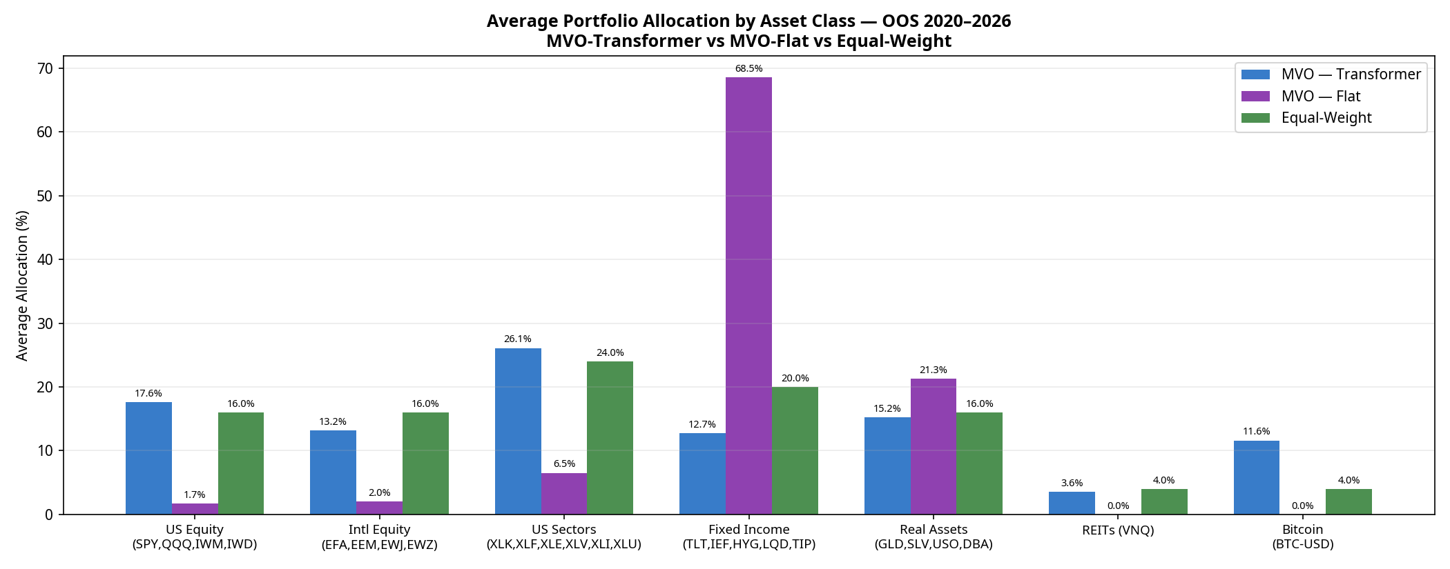
- MVO-Flat is dominated by Fixed Income (68.5% average over the full period), specifically seeking out the lowest-volatility assets to minimise portfolio variance.
- Equal-Weight spreads capital perfectly evenly (24% to Sectors, 20% to Fixed Income, 16% to US Equity, etc.).
- MVO-Transformer acts as a “risk-on” engine. Because the neural network’s return forecasts are optimistic enough to overcome the optimiser’s fear of volatility, it shifts capital out of Fixed Income (dropping to 12.7%) and heavily into US Sectors (26.1%), US Equities (17.6%), and notably, Bitcoin (11.6%).
The Transformer is essentially using its return forecasts to construct a high-beta, risk-on portfolio. When markets rally (2020, 2021, 2023–2026), it outperforms. When they crash (2022), it suffers.
6. Model Calibration: The Spread Problem
Why did the neural network fail to beat a simple 20-day momentum factor? The answer lies in the calibration of its predictions.
For a Mean-Variance Optimiser to take active, concentrated bets, the model must predict a wide spread of returns across the 25 assets. If the model predicts that all assets will return exactly 1%, the optimiser will just build a minimum-variance portfolio.
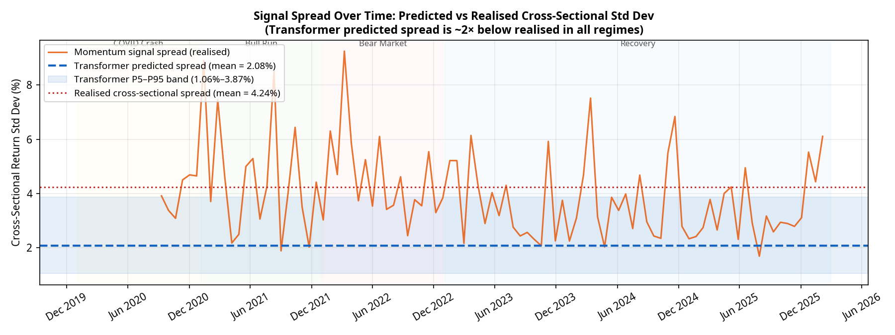
Our diagnostics show a severe and persistent calibration issue. Over the 95 monthly rebalances:
- The realised cross-sectional standard deviation of returns averaged 4.24%.
- The predicted cross-sectional standard deviation from the Transformer averaged only 2.08% (with a tight P5–P95 band of 1.06% to 3.87%).
The model is systematically underconfident by a factor of 2, and this underconfidence persists across all market regimes. Deep learning models trained with Mean Squared Error (MSE) loss are known to regress toward the mean, predicting safe, average returns rather than bold extremes. Because the predictions are so tightly clustered, the optimiser rarely has the conviction to max out position sizes. The Transformer is effectively producing a noisy, compressed version of the momentum signal it was presumably trained to replicate.
Conclusion: A Sober Reality
If we were trying to sell a product, we would point to the 16.3% CAGR, crop the chart to the 2023–2026 bull run, and declare victory.
But as quantitative researchers, the conclusion is different. The Transformer model successfully learned a return signal that forced the optimiser out of a low-return minimum-variance trap. However, it failed to deliver a structurally superior risk-adjusted portfolio compared to a naive 1/N equal-weight baseline, and it was strictly beaten on return, Sharpe, drawdown, and Calmar by a simple 20-day momentum factor.
The path forward isn’t necessarily a bigger neural network. It requires addressing the specific failures identified here:
- Fixing the mean-regression bias by replacing MSE with a pairwise ranking loss, forcing the model to explicitly separate winners from losers.
- Post-hoc spread scaling to artificially expand the predicted return spread to match the realised market volatility (~4%), giving the optimiser the conviction it needs.
- Dynamic covariance modelling (e.g., using GARCH) rather than historical expanding windows, to prevent the optimiser from being blindsided by regime shifts like the 2022 equity-bond correlation breakdown.
(Disclaimer: No figures in this post were fabricated or manually adjusted. All results are direct outputs of the backtest engine).
*Code for the full pipeline, including the PyTorch models and scipy optimisers, is available on GitHub: https://github.com/jkinlay/transformer_mvo_pipeline

Nicole Byers is an entertainment enthusiast! Nicole is an entertainment journalist for the Maple Grove Report.