Sony adds the Bravia Theater Bar 5 and Bar 7 to its soundbar lineup


Sony already has a robust collection of soundbars in its Bravia Theater lineup. Today, the company is adding two more, as well as new rear speakers and three new subwoofers. The Bar 7 will sit in Sony’s premium tier, alongside the existing (and larger) Bar 8 and Bar 9 models, while the Bar 5 will offer a more compact and more affordable solution just below the current Bar 6.

The Bravia Theater Bar 7 utilizes nine total drivers to produce Dolby Atmos, DTS:X and IMAX Enhanced sound. More specifically, that arrangement includes three woofers, two tweeters, two up-firing units and two side-firing drivers, in addition to four passive radiators. Compare that to the Bar 8 and Bar 9 which house 11 speakers and 13 speakers respectively. Sony says the Bar 7 has new two-way front speakers and the center, up-firing and side-firing drivers all have the company’s oval-shaped X-Balanced design. In terms of features, you get Sony’s 360 Spatial Sound Mapping and Sound Field Optimization for more immersive audio performance.

The Bar 7 will come bundled with Sony’s new Bravia Theater Sub 7 for $870, but you can also purchase it without the subwoofer (pricing TBA). For a more robust system, the Bar 7 can be paired with the company’s Bravia Theater Rear speakers.

Sony Bravia Theater Sub 7

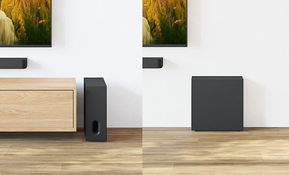
Sony Bravia Theater Sub 7 (Sony)

Speaking of subwoofers, Sony debuted three new models today. The aforementioned Sub 7 is the smallest, employing a 5.1-inch driver for the low-end tone. Move up to the new Sub 8 and you get a 7.9-inch driver for “enhanced atmosphere, clearer bass,” according to the company. The largest of the new options is the Sub 9 which has two opposing 7.9-inch drivers for “powerful, clean bass.” Unfortunately, these add-ons don’t come cheap: the Sub 7 is $330, the Sub 8 is $500 and the Sub 9 is $900.

Sony also touts dual subwoofer connectivity as part of the refreshed Bravia Theater lineup. All three of the new subs can be used as a pair, so long as you have a Theater Bar 7, Theater Bar 8 or Theater Bar 9. You can also use two subwoofers with some of Sony’s receivers (STR-AZ7000ES, STR-AZ5000ES, STR-AZ3000ES, STR-AZ1000ES and STR-AN1000). The company explains that opting for two subs provides “stronger, more balanced bass,” obviously, that fills the room for a more “cinematic effect.” Sony also says two subwoofers enable “richer, fuller bass” at lower volumes.

Rear speakers are something you’ll need if you truly want immersive audio, and the new Theater Rear 9 units are a big upgrade over the current Rear 8s. Most notably, you get an up-firing driver for enhanced overhead sounds along with two passive radiators, in addition to a tweeter and a woofer. The drivers all have aluminum diaphragms instead of paper, and the Rear 9s come with a swivel wall mounts that enable 60-degree movement. A pair of Theater Rear 9 speakers will set you back $750.

Sony Bravia Theater Bar 5

Sony Bravia Theater Bar 5 (Sony)

If all of that sounds too expensive for your living room, Sony has something more affordable in the midrange area. The Bravia Theater Bar 5 is just $350 and still offers Dolby Atmos and DTS:X audio. It doesn’t have up-firing drivers, it’s a 3.1-channel setup, so any overhead effects will be simulated. Still, that’s probably okay if you have a smaller space or live in an apartment as the upmixing tech (S-Force Pro Front Surround and Vertical Sound Engine) should provide ample immersion. The Bar 5 does come with a subwoofer though, and you can employ Sony’s Voice Zoom 3 feature for enhanced dialogue.

The Bravia Theater Bar 7, all three of the new subwoofers and the Rear 9 will be available for pre-order later this spring. The Bar 5 is up for pre-order starting today.


Source link

Leave a Reply

Subscribe to Our Newsletter

Get our latest articles delivered straight to your inbox. No spam, we promise.

Recent Reviews


Comparing the columns in Excel is a powerful way for analysing and understanding data and can help us in identifying the patterns and trends that we may not be able to find out through manual inspection. Using Excel formulas and techniques we can quickly and easily compare columns and gain insights that can help us in making better decisions. There are several ways to compare two columns in Excel. By using formulas like IF, COUNTIF, INDEX/MATCH and VLOOKUP. But before we compare we need to understand the type of data you are working with, like whether it is a numeric, text or date/time data. This will help you to choose the suitable tool or technique to compare it. For example if you are working with text data, you can use the IF function to compare and find the matching and non-matching entries. If you are working with numeric data, you may use a function like COUNTIF function to count the number of matching entries.

Methods to compare two columns in excel:

1. Using Equal operator

One of the simplest ways to compare values in two columns in Excel is using an equal operator. Let us understand how we can compare two columns using equal operators with an example.

  • First select a cell where you want to write the result
  • Then type “=” sign
  • Select the value in the first column which you want to compare then write “=” and select the value in another column and 
  • Hit the enter button


Want to gain knowledge in Excel? Then visit here to learn Excel Training!

Excel Training

  • Master Your Craft
  • Lifetime LMS & Faculty Access
  • 24/7 online expert support
  • Real-world & Project Based Learning

2. Using Conditional formatting:

a) Comparing two columns to highlight the duplicate values in the columns:

It is a feature in Excel that will highlight cells in one column that match/do not match with another column. To highlight the cells that have same values follow the below steps:

1. Select the two columns you want to compare.

2. Then go to the home tab and select the conditional formatting option.

3. Select the option Highlight cells Rules, then click on duplicate values option


4. Duplicate values dialogue box appears on the screen. Select an option from the dialogue box how the duplicate values must look like. In this Example I have chosen Green fill with dark green text. You can choose any option you like and click ok.

5. Then the duplicate text will be highlighted with green colour with dark green text

b) Comparing two columns to highlight the Unique values in the columns:

Now to highlight the cells that have different values follow the below steps:

  1. Select the two columns you want to compare.
  2. Then go to the home tab and select the conditional formatting option.
  3. Select the option Highlight cells Rules, then click on duplicate values option
  4. Duplicate values dialogue box appears on the screen. Select an option Unique instead of Duplicate from the dialogue box and also how the duplicate values must look like. In this Example I have chosen Light Red fill with dark Red text. You can choose any option you like and click ok.
  5. Then the unique text will be highlighted with light Red colour with dark Red text


Equal operator, Generals, compare-two-columns-in-excel-description-0, Generals, compare-two-columns-in-excel-description-0, Generals, compare-two-columns-in-excel-description-0, Equal operator, Generals, compare-two-columns-in-excel-description-0, Generals, compare-two-columns-in-excel-description-0, Equal operator, Generals, compare-two-columns-in-excel-description-0, , Generals, compare-two-columns-in-excel-description-1, Generals, compare-two-columns-in-excel-description-1, Generals, compare-two-columns-in-excel-description-1, Equal operator, Generals, compare-two-columns-in-excel-description-0, Generals, compare-two-columns-in-excel-description-0, Equal operator, Generals, compare-two-columns-in-excel-description-0, , Generals, compare-two-columns-in-excel-description-1, Generals, compare-two-columns-in-excel-description-1, Equal operator, Generals, compare-two-columns-in-excel-description-0, , Generals, compare-two-columns-in-excel-description-1, , Generals, compare-two-columns-in-excel-description-2, Generals, compare-two-columns-in-excel-description-2, Generals, compare-two-columns-in-excel-description-2

Subscribe to our YouTube channel to get new updates..!

3. Using Formulas

Excel offers a number of Formulas to compare the cells in two columns. Let us go through them one by one.

a) IF:

It allows you to compare two cells in two columns and will return the result based on the condition we provide. Let us understand how to use the IF formula to compare the values in two columns with an example.

  1. First select a cell where you want to write the result
  2. Then type “=” sign
  3. Type IF and open bracket “( and write the condition and put a comma. Then write the value to be displayed if the condition is true in inverted commas and put a comma, and then write the value to be displayed if the condition is false in inverted commas.
  4. Close the bracket “)” and hit the enter button


b) COUNTIF:

We can use this formula to compare the two columns and count the number of cells that are the same or different. Let us understand how to use the COUNTIF formula to compare the values in two columns with an example.

  1. First select a cell where you want to write the result
  2. Then type “=” sign
  3. Type COUNTIF and open bracket “(“ and select the range, put a comma and select the range from another column to compare it
  4. Close the bracket “)” and hit the enter button


Top 30 frequently asked Excel Interview Questions !

Excel Training

Weekday / Weekend Batches

c) MATCH:

We can use the match function to compare two columns and find the position of a value in one column that matches with the value in another column. Let us understand how to use the MATCH formula to compare the values in two columns with an example.

  1. First select a cell where you want to write the result
  2. Then type “=” sign
  3. Type MATCH and open bracket “(“ and select the cell which you wanted to compare, put a comma and select the range from another column to compare, put a comma and write 0 to get exact match
  4. Close the bracket “)” and hit the enter button


d) VLOOKUP:

We can use the VLOOKUP function for comparing two columns and return a value if there is a match. Let us understand how to use the VLOOKUP formula to compare the values in two columns with an example.

  1. First select a cell where you want to write the result
  2. Then type “=” sign
  3. Type VLOOKUP and open bracket “(“ and select the cell which you wanted to compare, put a comma and select the range from another column to compare, put a comma and write 2 to return the value from the second column of the range – if a match is found, put a comma and write FALSE to get exact match
  4. Close the bracket “)” and hit the enter button


Conclusion:

In this blog, We have discussed different ways to compare two columns in Excel with examples. We hope you found this information useful. For more information on Excel stay tuned.


Source link