
What is Big Data Modeling?
Data modeling is the method of constructing a specification for the storage of data in a database. It is a theoretical representation of data objects and relationships between them. The process of formulating data in a structured format in an information system is known as data modeling. It facilitates data analysis, which will aid in meeting business requirements.
Data modeling necessitates data modelers who will work closely with stakeholders and potential users of an information system. The data modeling method ends in developing a data model that supports the business information system’s infrastructure. This method also entails comprehending an organization’s structure and suggesting a solution that allows the organization to achieve its goals. It connects the technological and functional aspects of a project.
Why is Data Modeling necessary?
To ensure that we can easily access all books in a library, we must classify them and place them on racks. Likewise, if we have a lot of info, we’ll need a system or a process to keep it all organized. “Data modeling” refers to the method of sorting and storing data.”
A data model is a system for organizing and storing data. A data model helps us organise data according to service, access, and usage, just like the Dewey Decimal System helps us organise books in a library. Big data can benefit from appropriate models and storage environments in the following ways:
Performance: Good data models will help us quickly query the data we need and lower I/O throughput.
Cost: Good data models can help big data systems save money by reducing unnecessary data redundancy, reusing computing results, and lowering storage and computing costs.
Efficiency: Good data models can significantly enhance user experience and data utilization performance.
Quality: Good data models ensure that data statistics are accurate and that computing errors are minimized.
As a result, a big data system unquestionably necessitates high-quality data modeling methods for organizing and storing data, enabling us to achieve the best possible balance of performance, cost, reliability, and quality.
Why use a Data Model?
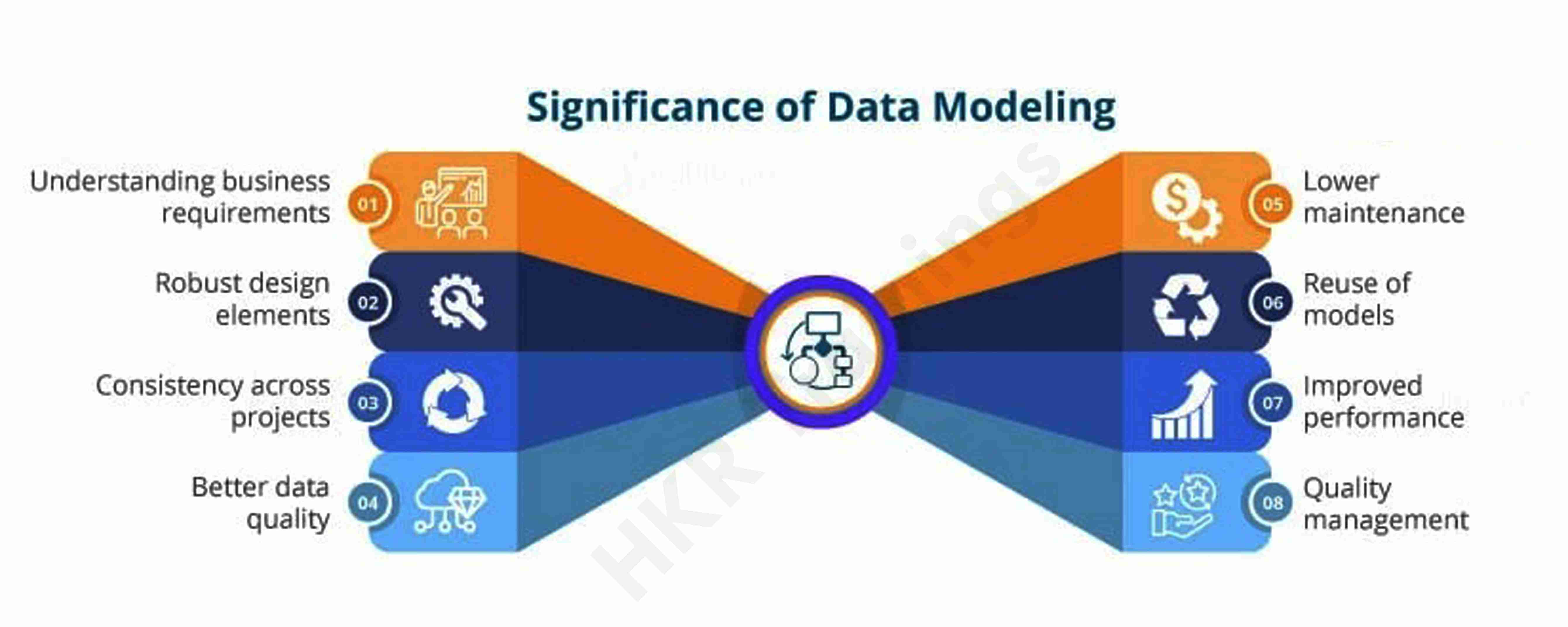
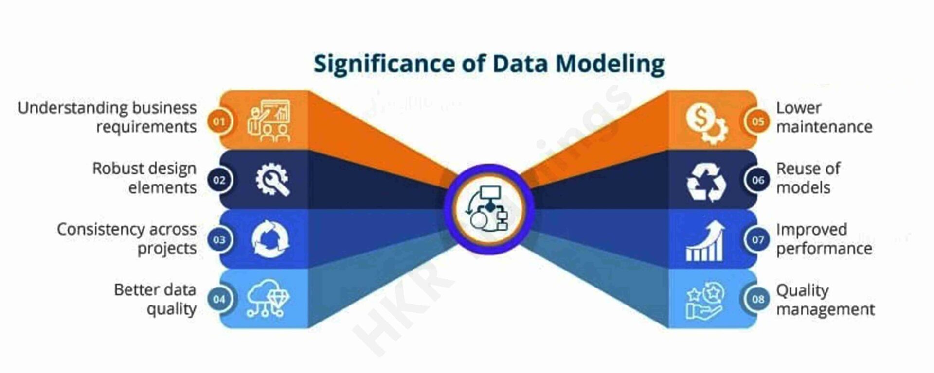
- Data interpretation can be improved by using a visual representation of the data. It gives developers a complete image of the data, which they can use to build a physical database.
- The model correctly depicts all of an organization’s essential data. Data omission is less likely thanks to the data model. Data omission can result in inaccurate results and reports.
- The data model depicts a clearer picture of market requirements.
- It aids in developing a tangible interface that unifies an organization’s data on a single platform. It also aids in the detection of redundant, duplicate, and incomplete data.
- A competent data model aids in ensuring continuity across all of an organization’s projects.
It enhances the data’s quality. - It aids Project Managers in achieving greater reach and quality control. It also boosts overall performance.
- Relational tables, stored procedures, and primary and foreign keys are all described in it.
Data Model Perspectives
Conceptual, logical, and physical data models are the three types of data models. Data models are used to describe data, how it is organized in a database, and how data components are related to one another.
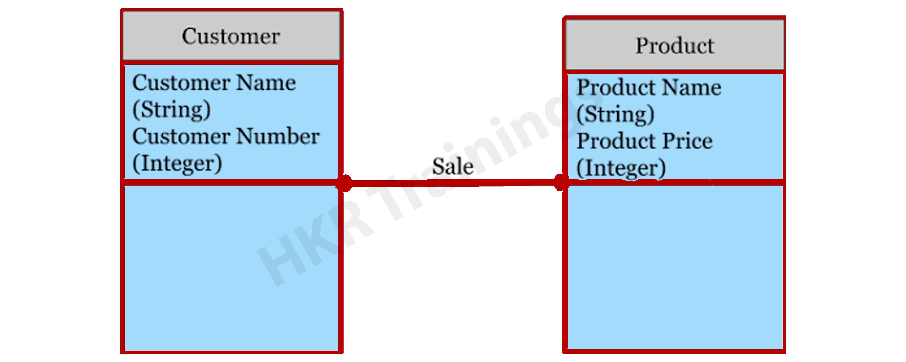
Conceptual Model
This stage specifies what must be included in the model’s configuration to describe and coordinate market principles. It focuses primarily on business-related entries, characteristics, and relationships. Data Architects and Business Stakeholders are mainly responsible for its development.
The Conceptual Data Model is used to specify the scope of the method. It’s a tool for organizing, scoping, and visualizing company ideas. The aim of developing a computational data model is to develop new entities, relationships, and attributes. Data architects and stakeholders typically create a computational data model.
The Conceptual Data Model is held by three key holders.
- Entity: A real-life thing
- Attribute: Properties of an entity
- Relationship: Association between two entities
Let’s take a look at an illustration of this data model.
Consider the following two entities: product and customer. The Product entity’s attributes are the name and price of the product, while the Customer entity’s attributes are the name and number of customers. Sales is the connection between these two entities.
- The Conceptual Data Model was created with a corporate audience in mind.
- It offers an overview of corporate principles for the whole organization.
- It is created separately, with hardware requirements such as location and data storage space and software requirements such as technology and DBMS vendor.

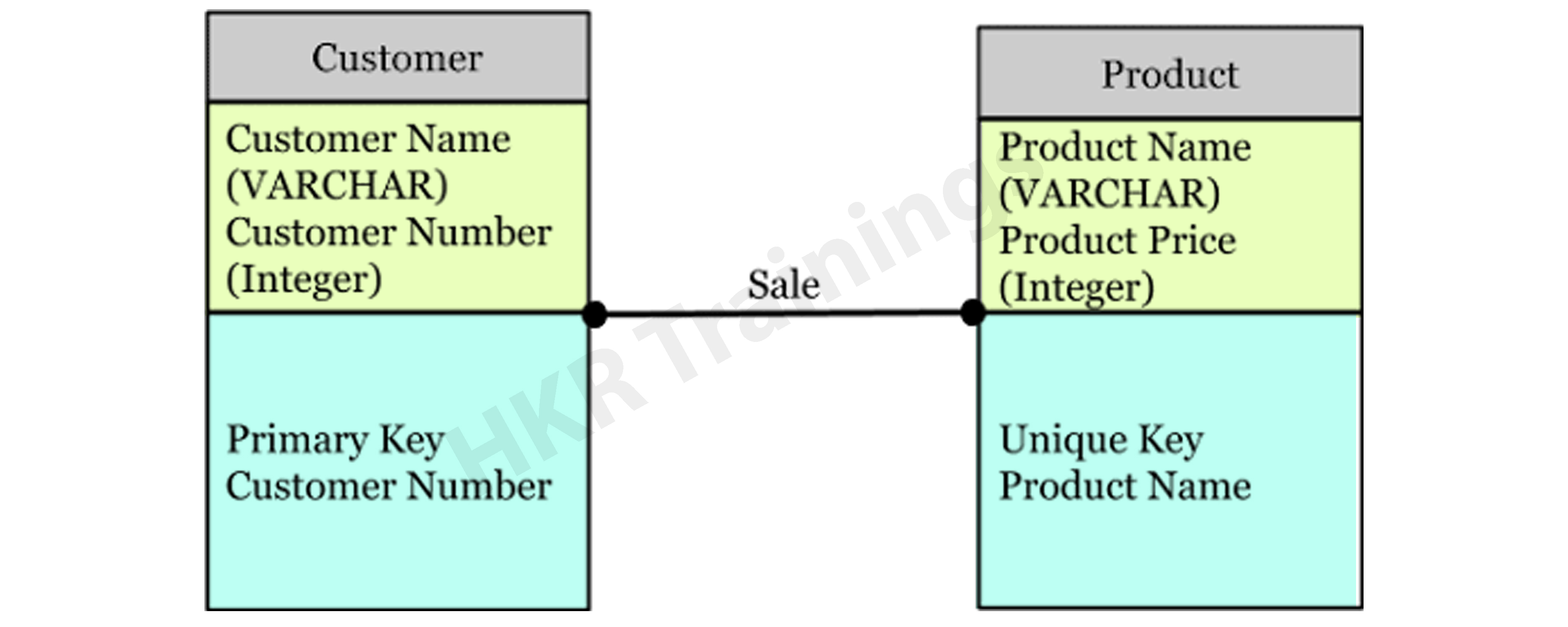
Logical Model
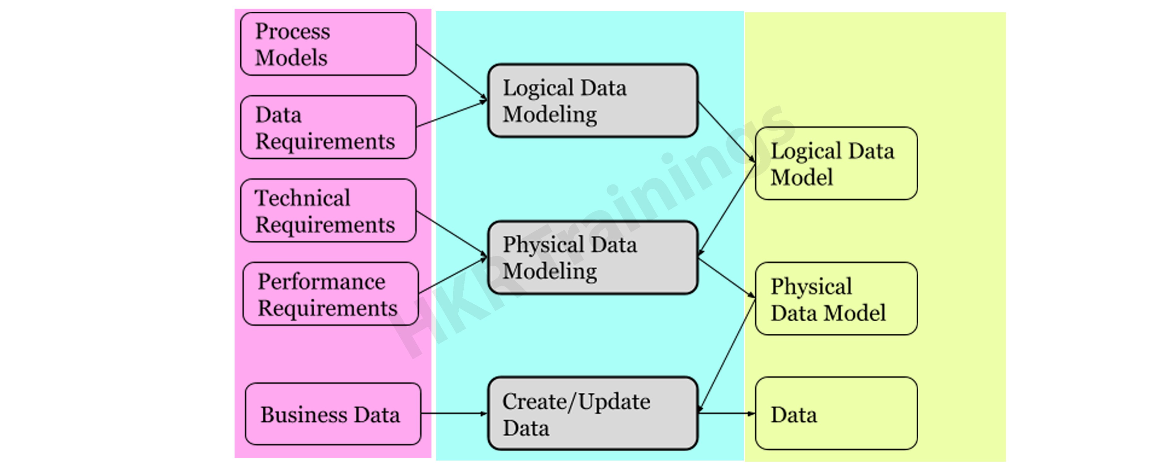
The conceptual model lays out how the model can be put into use. It encompasses all types of data that must be captured, such as tables, columns, and so on. Business Analysts and Data Architects are the most prominent designers of this model.
The Logical Data Model is used to describe the arrangement of data structures as well as their relationships. It lays the groundwork for constructing a physical model. This model aids in the inclusion of extra data to the conceptual data model components. There is no primary or secondary key specified in this model. This model helps users to update and check the connector information for relationships that have been set previously.
The logical data model describes the data requirements for a single project, but it may be combined with other logical data models depending on the project’s scope. Data attributes come with a variety of data types, many of which have exact lengths and precisions.
- The logical data model is created and configured separately from the database management system.
- Data Types with accurate dimensions and precisions exist for data attributes.
- It specifies the data needed for a project but, depending on the project’s complexity, interacts with other logical data models.
Top 80+ frequently asked Data Modeling Interview questions!

Big Data Hadoop Training
- Master Your Craft
- Lifetime LMS & Faculty Access
- 24/7 online expert support
- Real-world & Project Based Learning
Physical Model
The physical model explains how to use a database management system to execute a data model. It lays out the process in terms of tables, CRUD operations, indexes, partitioning, etc. Database Administrators and Developers build it.
The Physical Data Model specifies how a data model is implemented in a database. It attracts databases and aids in developing schemas by duplicating database constraints, triggers, column keys, other RDBMS functions, and indexes. This data model aids in visualizing the database layout. Views, access
profiles, authorizations, primary and foreign keys, and so on are all specified in this model.
The majority and minority relationships are defined in the Data Model by the relationship between tables. It is created for a specific version of a database management system, data storage, and project site.
- The Physical Data Model was created for a database management system (DBMS), data storage, and a project site.
- It contains table relationships that address the nullability and cardinality of the relationships.
- Views, access profiles, authorizations, primary and foreign keys, and so on are all specified here.
Realted Article: CAP Theorem in Big Data!
Types of Data Models
While there are several different data modeling approaches, the basic principle remains the same with all models. Let’s take a look at some of the most commonly used data models:
Hierarchical Model
This is a database modeling technique that uses a tree-like structure to organise data. Each record in this table has a single root or parent. When it comes to sibling documents, they’re organized in a specific way. This is the physical order in which the information is stored. This method of modeling can be applied to a wide range of real-world model relationships. This database model was popular in the 1960s and 1970s. However, owing to inefficiencies, they are still used infrequently.
The hierarchical model is used to assemble data into a tree-like structure with a single root that connects all of the data. A single root like this evolves like a branch, connecting nodes to the parent nodes, with each child node having just one parent node. The data is structured in a relational system with a one-to-many relationship between two different data types in this model. For example, in a college, a department consists of a set of courses, professors, and students.

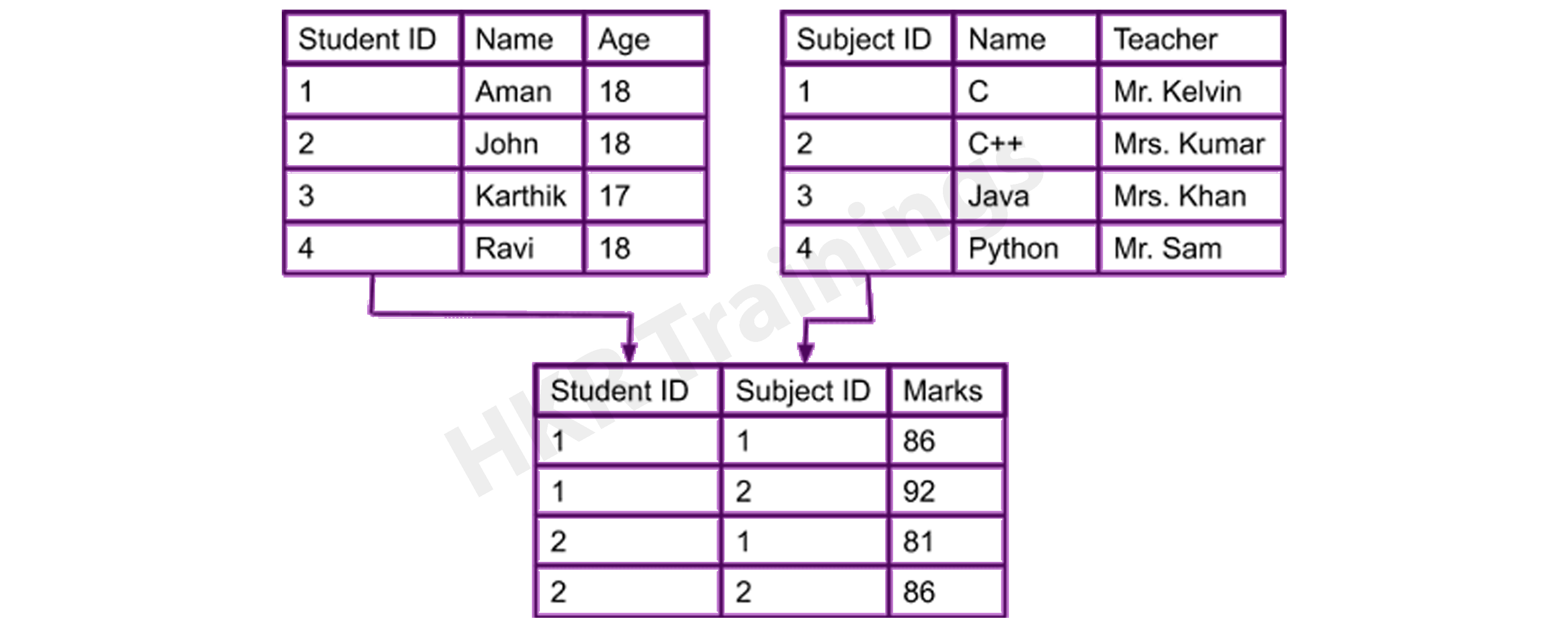
Relational Model
In 1970, an IBM researcher suggested this as a possible solution to the hierarchical paradigm. The data path does not need to be defined by developers. Tables are used to merge data segments in this case directly. The program’s complexity has been minimized due to this model. It necessitates a thorough understanding of the organization’s physical data management strategy. This model was quickly merged with Structured Query Language after its introduction (SQL).
A typical field maintains the Relational Model aids in the organization of two-dimensional tables and the interaction. Tables are the data structure of a relational data model. The table’s rows contain all of the information for a given category. In the Relational Model, these tables are referred to as relations.
Network Model
The Network Model is an enhancement of the Hierarchical Model, allowing for various relationships with related records, implying multiple parent records. It will enable users to build models using sets of similar documents following mathematical set theory. A parent record and the number of child records are included in this set. Each record is a member of several sets, allowing the model to define complex relationships. The model can express complex relationships since each record can belong to several sets.

Object-oriented Database Model
A set of objects are aligned with methods and functions in the Object-oriented Database. There are characteristics and methods associated with these objects. Multimedia databases, hypertext databases, and other types of object-oriented databases are available. Even if it incorporates tables, this type of database model is known as a post-relational database model since it is not limited to tables. These database models are referred to as hybrid models.
Wish to make a career in the world of Datastage? Start with Datastage Online Training!

Subscribe to our YouTube channel to get new updates..!
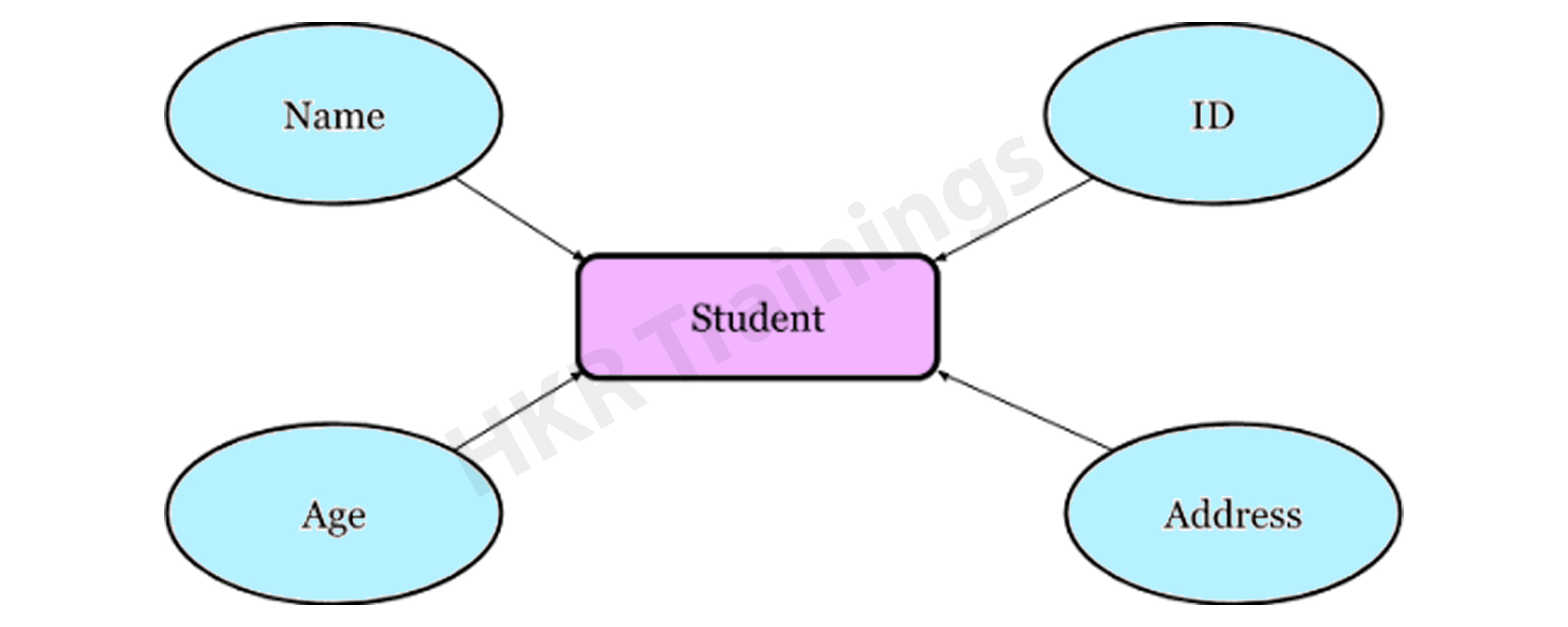
Entity–Relationship Model
The Entity-Relationship Model (ERM) is a diagram that depicts entities and their relationships. The E-R model generates an entity set, attributes, relationship set, and constraints when constructing a real-world scenario database model. The E-R diagram is a graphical representation of this kind.
An entity may be an object, a concept, or a piece of data stored in relation to the data. It has properties called attributes, and a set of values called domain defines each attribute. A relationship is a logical connection between two or more entities. These connections are mapped to entities in several ways.
Consider a College Database, where a Student is an entity, and the Attributes are Student details such as Name, ID, Age, Address, and so on. As a result, there will be a relation between them.
Object-relational Model
The object-relational model can be thought of as a relational model with enhanced object-oriented database model features. This kind of database model enables programmers to integrate functions into a familiar table structure.
An Object-relational Data Model combines the advantages of both an Object-oriented and a Relational database model. It supports classes, objects, inheritance, and other features similar to the Object-oriented paradigm and data types, tabular structures, and other features similar to the Relational database model. Designers may use this model to integrate functions into table structures.
Facts and Dimensions
To understand data modelling, one must first grasp its facts and dimensions.
Fact Table: It’s a table that lists all of the measurements and their granularity. Sales, for example, maybe additive or semi-additive.
Dimension Table: It’s a table containing fields with definitions of market elements and is referenced by several fact tables.
Dimensional Modeling: Dimensional modeling is a data warehouse design methodology. It makes use of validated measurements and facts and aids in navigation. The use of dimensional modeling in performance queries speeds up the process. Star schemas are a colloquial term for dimensional models.
Dimensional Modeling-Related Keys
While learning data modeling, it’s critical to understand the keys. There are five different types of dimensional modelling keys.
- Business or Natural Keys: It is a field that uniquely defines an individual. Customer ID, employee number, and so on.
- Primary and Alternate Keys: A primary key is an area that contains a single unique record. The consumer must choose one of the available primary keys, with the others being alternative keys.
- Composite or Compound Keys: A composite key is one in which more than one field is used to represent a key.
- Surrogate Keys: It is usually an auto-generated field with no business meaning.
- Foreign Keys: It is a key that refers to another key in some other table.
The process of data modeling entails the development and design of various data models. A data definition language is then used to convert these data models. A database is created using a data definition language. This database will be referred to as a wholly attributed data model at that stage.
Benefits and Drawbacks of Data Models
Benefits:
- With data modeling, the functional team’s data objects are appropriately presented.
- Data modeling enables you to query data from a database and generate various reports from it. With the aid of reports, it indirectly contributes to data analysis. These reports can be used to improve the project’s quality and efficiency.
- Businesses have a large amount of data in various formats. For such unstructured data, data modeling offers a structured framework.
- Data modeling enhances business intelligence by requiring data modelers to work closely with the project’s realities, such as data collection from various unstructured sources, reporting specifications, spending patterns, and so on.
- It improves coordination within the business.
- The documentation of data mapping is aided during the ETL method.
Drawbacks:
- The development of a data model is a time-consuming process. Should understand the physical characteristics of data storage.
- This method necessitates complex application creation as well as biographical truth information.
- The model isn’t particularly user-friendly. Small improvements in the method require a significant rewrite of the entire application.
Big Data Hadoop Training
Weekday / Weekend Batches
Conclusion
Data models are created to store data in a database. The primary goal of these data models is to ensure that the data objects generated by the functional team are correctly denoted. As previously stated, even the little improvement in the system necessitates improvements to the entire model. Despite the problems, the data modelling concept is the first and most important step of database design since it describes data entities, relationships between data objects, and so on. A data model discusses the data’s market rules, government regulations, and regulatory enforcement in a holistic manner.
Related Article:

Stephan is the sports journalist for the Maple Grove Report.