Marcel Hug wins 9th Boston Marathon wheelchair title


Marcel Hug

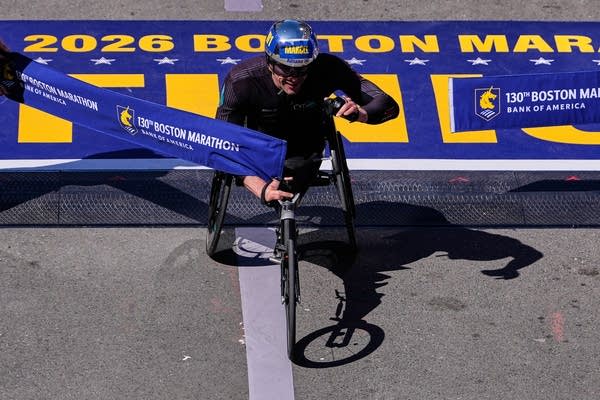
Marcel Hug of Switzerland won his ninth Boston Marathon wheelchair title on Monday, riding a tailwind to finish in an unofficial time of 1 hour, 16 minutes, 6 seconds. He missed breaking his own course record by 33 seconds.

Two-time winner Daniel Romanchuk of Champaign, Illinois, was second behind Hug for the fourth straight time.

In the women's wheelchair race, Eden Rainbow-Cooper won for the second time, finishing in an unofficial 1:30:51 to beat runner-up Catherine Debrunner of Switzerland by more than two minutes.

The fastest field in event history and ideal weather had runners expecting fast times in the 130th edition of the world's oldest and most prestigious annual marathon.

The athletes arrived in Hopkinton with frost on the ground and temperatures in the 30s. It had warmed to 45 degrees (7 degrees Celsius) by the the time defending champions Sharon Lokedi and John Korir started the race, followed by more than 30,000 others.

It was the coldest starting temperature since 2018, when it was 38 degrees and raining. Last year, the thermostat was at 58 when runners set off.

Military marchers and 50 wheelchair athletes were first over the starting line, with the men's and women's fields following. Lokedi, who shattered the women's course record last year, is back, and Korir goes for another win in the men's race a year after posting the third-fastest time in Boston history.

On the 50th anniversary of the “Run for the Hoses,” when Jack Fultz won in temperatures approaching 100 degrees (38 degrees Celsius), cool weather greeted the runners in Hopkinton and was expected to reach into the 40s during the day.

Fultz, who was serving as grand marshal, said as he waited to board his ride that the weather was the “polar opposite” from the day of his 1976 win.

“I am just trying to soak it all in, to remember it all," he said. “There are almost are no words to fully describe the kind of experience. You have a dream of a lifetime and all of a sudden it comes true.”

A tailwind was expected to help the competitors as they make their way to Boston's Back Bay.

Runners may notice some changes this year, with the race turning to a crowd scientist for help in spreading things out a little so they don’t face bottlenecks on the narrow streets of the eight cities and towns along the course. At the start is a new statue of and by marathon pioneer Bobbi Gibb — the first statue on the course honoring a woman.

Race Director Dave McGillivray sent the group of about 50 members of the Massachusetts National Guard members off at 6 a.m. McGillivray said it's the coldest start he could remember in his nearly four decades working at the race.

Staff Sgt. Mackenzie Smith and Spec. Benjamin De Boer stepped back and forth to try to stay warm before they set off on the course, but the cold didn't dampen their enthusiasm for participating in the Boston Marathon for the first time.

“It's an honor and a blessing to be standing at the Boston Marathon start,” Smith said. “The history that goes with the marathon resonates with me, growing up in Massachusetts.”

McGillivray said the cold added another layer of complexity because runners were arriving in Hopkinton with many layers of extra clothing that would be discarded at the start line and need to be collected. But as the sun comes out, he said it will be ideal for running.


Source link

Leave a Reply

Subscribe to Our Newsletter

Get our latest articles delivered straight to your inbox. No spam, we promise.

Recent Reviews


Comparing the columns in Excel is a powerful way for analysing and understanding data and can help us in identifying the patterns and trends that we may not be able to find out through manual inspection. Using Excel formulas and techniques we can quickly and easily compare columns and gain insights that can help us in making better decisions. There are several ways to compare two columns in Excel. By using formulas like IF, COUNTIF, INDEX/MATCH and VLOOKUP. But before we compare we need to understand the type of data you are working with, like whether it is a numeric, text or date/time data. This will help you to choose the suitable tool or technique to compare it. For example if you are working with text data, you can use the IF function to compare and find the matching and non-matching entries. If you are working with numeric data, you may use a function like COUNTIF function to count the number of matching entries.

Methods to compare two columns in excel:

1. Using Equal operator

One of the simplest ways to compare values in two columns in Excel is using an equal operator. Let us understand how we can compare two columns using equal operators with an example.

  • First select a cell where you want to write the result
  • Then type “=” sign
  • Select the value in the first column which you want to compare then write “=” and select the value in another column and 
  • Hit the enter button


Want to gain knowledge in Excel? Then visit here to learn Excel Training!

Excel Training

  • Master Your Craft
  • Lifetime LMS & Faculty Access
  • 24/7 online expert support
  • Real-world & Project Based Learning

2. Using Conditional formatting:

a) Comparing two columns to highlight the duplicate values in the columns:

It is a feature in Excel that will highlight cells in one column that match/do not match with another column. To highlight the cells that have same values follow the below steps:

1. Select the two columns you want to compare.

2. Then go to the home tab and select the conditional formatting option.

3. Select the option Highlight cells Rules, then click on duplicate values option


4. Duplicate values dialogue box appears on the screen. Select an option from the dialogue box how the duplicate values must look like. In this Example I have chosen Green fill with dark green text. You can choose any option you like and click ok.

5. Then the duplicate text will be highlighted with green colour with dark green text

b) Comparing two columns to highlight the Unique values in the columns:

Now to highlight the cells that have different values follow the below steps:

  1. Select the two columns you want to compare.
  2. Then go to the home tab and select the conditional formatting option.
  3. Select the option Highlight cells Rules, then click on duplicate values option
  4. Duplicate values dialogue box appears on the screen. Select an option Unique instead of Duplicate from the dialogue box and also how the duplicate values must look like. In this Example I have chosen Light Red fill with dark Red text. You can choose any option you like and click ok.
  5. Then the unique text will be highlighted with light Red colour with dark Red text


Equal operator, Generals, compare-two-columns-in-excel-description-0, Generals, compare-two-columns-in-excel-description-0, Generals, compare-two-columns-in-excel-description-0, Equal operator, Generals, compare-two-columns-in-excel-description-0, Generals, compare-two-columns-in-excel-description-0, Equal operator, Generals, compare-two-columns-in-excel-description-0, , Generals, compare-two-columns-in-excel-description-1, Generals, compare-two-columns-in-excel-description-1, Generals, compare-two-columns-in-excel-description-1, Equal operator, Generals, compare-two-columns-in-excel-description-0, Generals, compare-two-columns-in-excel-description-0, Equal operator, Generals, compare-two-columns-in-excel-description-0, , Generals, compare-two-columns-in-excel-description-1, Generals, compare-two-columns-in-excel-description-1, Equal operator, Generals, compare-two-columns-in-excel-description-0, , Generals, compare-two-columns-in-excel-description-1, , Generals, compare-two-columns-in-excel-description-2, Generals, compare-two-columns-in-excel-description-2, Generals, compare-two-columns-in-excel-description-2

Subscribe to our YouTube channel to get new updates..!

3. Using Formulas

Excel offers a number of Formulas to compare the cells in two columns. Let us go through them one by one.

a) IF:

It allows you to compare two cells in two columns and will return the result based on the condition we provide. Let us understand how to use the IF formula to compare the values in two columns with an example.

  1. First select a cell where you want to write the result
  2. Then type “=” sign
  3. Type IF and open bracket “( and write the condition and put a comma. Then write the value to be displayed if the condition is true in inverted commas and put a comma, and then write the value to be displayed if the condition is false in inverted commas.
  4. Close the bracket “)” and hit the enter button


b) COUNTIF:

We can use this formula to compare the two columns and count the number of cells that are the same or different. Let us understand how to use the COUNTIF formula to compare the values in two columns with an example.

  1. First select a cell where you want to write the result
  2. Then type “=” sign
  3. Type COUNTIF and open bracket “(“ and select the range, put a comma and select the range from another column to compare it
  4. Close the bracket “)” and hit the enter button


Top 30 frequently asked Excel Interview Questions !

Excel Training

Weekday / Weekend Batches

c) MATCH:

We can use the match function to compare two columns and find the position of a value in one column that matches with the value in another column. Let us understand how to use the MATCH formula to compare the values in two columns with an example.

  1. First select a cell where you want to write the result
  2. Then type “=” sign
  3. Type MATCH and open bracket “(“ and select the cell which you wanted to compare, put a comma and select the range from another column to compare, put a comma and write 0 to get exact match
  4. Close the bracket “)” and hit the enter button


d) VLOOKUP:

We can use the VLOOKUP function for comparing two columns and return a value if there is a match. Let us understand how to use the VLOOKUP formula to compare the values in two columns with an example.

  1. First select a cell where you want to write the result
  2. Then type “=” sign
  3. Type VLOOKUP and open bracket “(“ and select the cell which you wanted to compare, put a comma and select the range from another column to compare, put a comma and write 2 to return the value from the second column of the range – if a match is found, put a comma and write FALSE to get exact match
  4. Close the bracket “)” and hit the enter button


Conclusion:

In this blog, We have discussed different ways to compare two columns in Excel with examples. We hope you found this information useful. For more information on Excel stay tuned.


Source link