Comparing the columns in Excel is a powerful way for analysing and understanding data and can help us in identifying the patterns and trends that we may not be able to find out through manual inspection. Using Excel formulas and techniques we can quickly and easily compare columns and gain insights that can help us in making better decisions. There are several ways to compare two columns in Excel. By using formulas like IF, COUNTIF, INDEX/MATCH and VLOOKUP. But before we compare we need to understand the type of data you are working with, like whether it is a numeric, text or date/time data. This will help you to choose the suitable tool or technique to compare it. For example if you are working with text data, you can use the IF function to compare and find the matching and non-matching entries. If you are working with numeric data, you may use a function like COUNTIF function to count the number of matching entries.
Methods to compare two columns in excel:
1. Using Equal operator
One of the simplest ways to compare values in two columns in Excel is using an equal operator. Let us understand how we can compare two columns using equal operators with an example.
- First select a cell where you want to write the result
- Then type “=” sign
- Select the value in the first column which you want to compare then write “=” and select the value in another column and
- Hit the enter button
-
![]()
Want to gain knowledge in Excel? Then visit here to learn Excel Training!
Excel Training
- Master Your Craft
- Lifetime LMS & Faculty Access
- 24/7 online expert support
- Real-world & Project Based Learning
2. Using Conditional formatting:
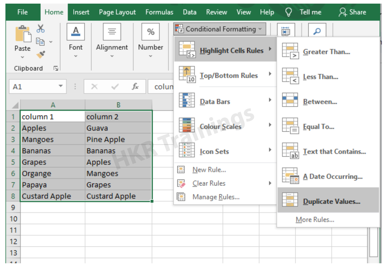
a) Comparing two columns to highlight the duplicate values in the columns:
It is a feature in Excel that will highlight cells in one column that match/do not match with another column. To highlight the cells that have same values follow the below steps:
1. Select the two columns you want to compare.
2. Then go to the home tab and select the conditional formatting option.
3. Select the option Highlight cells Rules, then click on duplicate values option
![]()
4. Duplicate values dialogue box appears on the screen. Select an option from the dialogue box how the duplicate values must look like. In this Example I have chosen Green fill with dark green text. You can choose any option you like and click ok.
5. Then the duplicate text will be highlighted with green colour with dark green text
![]()
b) Comparing two columns to highlight the Unique values in the columns:
Now to highlight the cells that have different values follow the below steps:
- Select the two columns you want to compare.
- Then go to the home tab and select the conditional formatting option.
- Select the option Highlight cells Rules, then click on duplicate values option
- Duplicate values dialogue box appears on the screen. Select an option Unique instead of Duplicate from the dialogue box and also how the duplicate values must look like. In this Example I have chosen Light Red fill with dark Red text. You can choose any option you like and click ok.
- Then the unique text will be highlighted with light Red colour with dark Red text
![]()
Subscribe to our YouTube channel to get new updates..!
3. Using Formulas
Excel offers a number of Formulas to compare the cells in two columns. Let us go through them one by one.
a) IF:
It allows you to compare two cells in two columns and will return the result based on the condition we provide. Let us understand how to use the IF formula to compare the values in two columns with an example.
- First select a cell where you want to write the result
- Then type “=” sign
- Type IF and open bracket “(” and write the condition and put a comma. Then write the value to be displayed if the condition is true in inverted commas and put a comma, and then write the value to be displayed if the condition is false in inverted commas.
- Close the bracket “)” and hit the enter button
![]()
b) COUNTIF:
We can use this formula to compare the two columns and count the number of cells that are the same or different. Let us understand how to use the COUNTIF formula to compare the values in two columns with an example.
- First select a cell where you want to write the result
- Then type “=” sign
- Type COUNTIF and open bracket “(“ and select the range, put a comma and select the range from another column to compare it
- Close the bracket “)” and hit the enter button
![]()
Top 30 frequently asked Excel Interview Questions !
Excel Training
Weekday / Weekend Batches
c) MATCH:
We can use the match function to compare two columns and find the position of a value in one column that matches with the value in another column. Let us understand how to use the MATCH formula to compare the values in two columns with an example.
- First select a cell where you want to write the result
- Then type “=” sign
- Type MATCH and open bracket “(“ and select the cell which you wanted to compare, put a comma and select the range from another column to compare, put a comma and write 0 to get exact match
- Close the bracket “)” and hit the enter button
![]()
d) VLOOKUP:
We can use the VLOOKUP function for comparing two columns and return a value if there is a match. Let us understand how to use the VLOOKUP formula to compare the values in two columns with an example.
- First select a cell where you want to write the result
- Then type “=” sign
- Type VLOOKUP and open bracket “(“ and select the cell which you wanted to compare, put a comma and select the range from another column to compare, put a comma and write 2 to return the value from the second column of the range – if a match is found, put a comma and write FALSE to get exact match
- Close the bracket “)” and hit the enter button
Conclusion:
In this blog, We have discussed different ways to compare two columns in Excel with examples. We hope you found this information useful. For more information on Excel stay tuned.